In Flood Risk Modeling, Resolution Matters – Even When You Think It Shouldn’t

This post is part of a series sponsored by CoreLogic.

We have all seen the dramatic pictures of destruction and loss after a devastating flood event. Usually, the scene is depicted as a sea of water inundating broad areas of a geographic region, impacting communities and homes. However, what we usually don’t understand from these images is the significant regional variations of water depth. This is one of the key indicators of contents and building damage, and therefore integral to understanding flood modeling.

Spatial resolution is important when measuring flood risk. While the underlying flood science and hazard data resolution is key, one of the most significant factors for accurately assessing flood risk is the site elevation relative to surface water elevation. Determining site elevation often requires parcel or building-level geocoding to obtain the location accuracy required to model flood risk. In addition to location accuracy, modeling with the optimal elevation data resolution is also critical. The following examples explore the impact that less than one meter in elevation and location accuracy can have on modeled loss.

A public study compiled by the North Carolina Geospatial & Technology Management Office in coordination with the North Carolina Department of Transportation highlights the importance of high resolution elevation data to expertly model flood risk. More importantly, it shows the potential for dramatically underestimating or, in some cases, overestimating risk¹. Below are two images from the study.

Figure 1

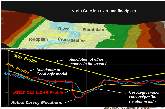
The yellow line in the top image delineates the location of the cross section shown in the second image of a river channel in North Carolina. Manual elevation survey points are depicted by the grey dots. These are somewhat obscured by the red line, which is the QL2 profile that shows the quality level 2 light detection and ranging elevation (LiDAR) data. The latter is the current standard acquired by the United States Geological Survey (USGS) with 20 centimeters vertical resolution for non-vegetated cover and 30 centimeters for vegetated cover. As you can see, there is a strong match between the two surveys. The blue line represents a 4-meter resolution profile, while the orange line represents a 10-meter resolution profile. The latter is the elevation resolution available consistently across the lower 48 states in the U.S., and although 3-meter resolution data is also available, it is not consistent across the country. Both the 4-meter and the 10-meter resolution cross sections in this example track fairly consistently with the river channel profile.

For additional comparison, the 30-meter resolution digital elevation is depicted in yellow. Several flood models currently on the market incorporate this lower resolution, but as illustrated, they do not accurately define the actual profile of the river channel and floodplain. As such, models using this 30-meter resolution data could vastly underestimate or overestimate the risk along this profile.

Consistency from Underwriting to Portfolio Management
With the flood insurance market poised for growth, one common concern CoreLogic® hears is that there is no adequate loss model to characterize the risk from site-specific underwriting through to portfolio management. Accuracy in location, hazard, vulnerability and financial model component resolution is critical for this peril in order to adequately model loss. Furthermore, accuracy at the site level not only improves underwriting confidence, but also leads to greater accuracy in determining aggregate risk.

The following example expands on the previous North Carolina sample and provides insight into the impact of spatial accuracy relative to modeled loss. Similar to Figure 1, Figure 2 shows a cross section of the Arroyo de la Laguna watercourse which extends the length of the city of Pleasanton, California, in the eastern portion of the San Francisco Bay Area, and ultimately drains into the San Francisco Bay. This region has a historical record of flooding, with the largest flood between December 22 and December 24, 1955 fully inundating the northern part of the region—which back then was mostly farmland. This flood was caused by a series of devastating storms that impacted a broad region along the west coast of the U.S. Total deaths due to the storms across the entire west coast was 67 with direct losses of $1.7B in 2016 dollars.² While no deaths were recorded in the Pleasanton region, the series of storms caused 31 deaths in the seven county San Francisco Bay Area with total property damage that was estimated at over $75M (or approximately $670M in 2016 dollars)².

Since then, Pleasanton has undergone exponential growth to become a significant urban region with high density residential and commercial developments. For example, upstream dam construction in 1968 and drainage alterations performed on the watercourse reduced flood risk; however, it has still been subject to flooding, with the most recent event in 1988 causing significant flooding in localized areas. It is important to note that a large component of this recent flood event was caused by flash flooding, not just riverine flooding. Figure 2 also shows that the Federal Emergency Management Agency (FEMA) 100-year flood zone boundary matches the width of the waterway channel even though flooding potential—and especially flash flooding potential—has historically not been constrained to this boundary.

Figure 2

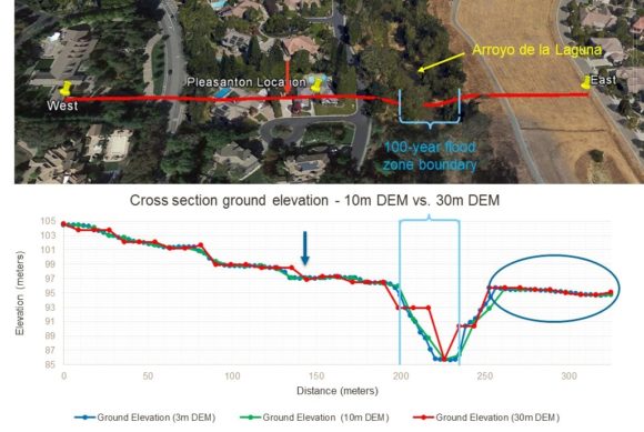
Unlike the previous example, sites at 10-meter intervals have been created along the cross section. These are analyzed to illustrate the impact on loss of elevation assignments relative to both 10-meter and 30-meter digital elevation model (DEM) data. The elevation cross section in Figure 2 shows 3-meter, 10-meter and 30-meter DEM data results. Notable is that both the 3-meter and 10-meter DEM profiles match one another well. However, the 30-meter DEM profile shows significant differences, especially at the location of the arrow, where the graded ground elevation changes from one property to another, as well as along the watercourse channel. The elevation differences are also less along flat regions as seen on the right side of the cross section. But, when we ask if this will this translate to similar loss potential, the answer is “not always.”

For illustrative purposes, a $1 million combined structure and contents reconstruction cost value (construction costs can be over $250 per square foot in this region) was modeled at each “site” with the CoreLogic probabilistic U.S. Inland Flood Model at 10-meter intervals along the cross section. Both the 10-meter and 30-meter DEM data were used in the analysis. Figure 3 shows the modeled mean annual loss, the common basis for assessing premium needed to cover loss over time. At the location marked by the arrow that was referenced earlier, the 10-meter DEM results in a $339 higher pure premium than the 30-meter DEM result – a 33 percent difference. This result could have an impact on both risk selection and pricing.

Figure 3

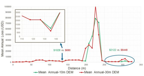
Focusing on the right side of the cross section, we see that despite the similarity in ground elevation for each of the DEMs, there is a significant loss difference. This is driven by the differences in the channel geometry defined by the 10-meter versus 30-meter DEM data, as well as the downward slope of the topography away from the channel edge up to the berm. The 30-meter channel is narrower at depth, which reduces the volume of water that the channel can hold and increases the velocity of the water. These conditions increase water depth and damage potential, leading to greater loss where water banks up against the higher elevation starting at the endpoint of the cross section.

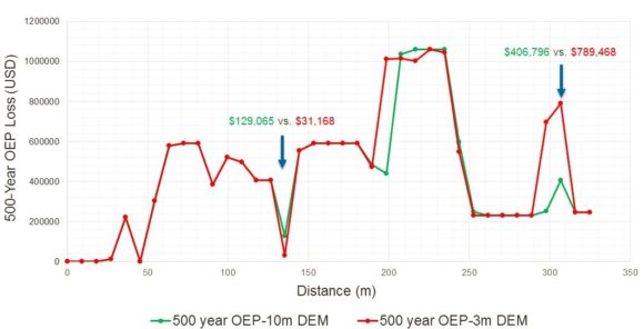
The graph in Figure 4 shows the loss differences at the 500-year loss return period, or the probability of meeting or exceeding the 500-year loss threshold from at least one event in any year. This is distinct from a 500-year flood (being attributed to much of the flooding in the summer of 2016), which denotes that a flood event has a 0.2 percent chance of occurring in any given year. Note that the same loss pattern is repeated, but the loss differences are much greater with a $97,897 difference in loss near the 140-meter location, or a 76 percent loss difference.

Figure 4

This example illustrates the potential impact of data accuracy and resolution on not just hazard assessment, but on loss modeling as well—both critical input to accurately managing flood-exposed risks at the site as well as when aggregated to the account or portfolio level.

Flood risk in the U.S. continues to be a significant and growing insured loss threat to the private insurance industry, whether as a policy endorsement, a named peril or an inclusion in a multi-peril policy. As the private insurance industry explores diversifying and growing business with the potential changes in National Flood Insurance Program (NFIP) coverage and rates, as well as an increased perception of risk, insurers are seeking highly granular loss models to address the management of a peril where the amount of loss can be largely influenced by small variations in water depth. Therefore, it is extremely important that insurers leverage data that is current, detailed and highly granular for sound flood risk assessment.

Sources:

1. 2014 LiDAR Collection – Coordination across Federal and State Data Collections, Geospatial and Technology Management, Feb 18, 2014.

http://www.ncfloodmaps.com/pubdocs/lidar_onepager.pdf

2. Blodgett, J.C. and Chin, Edwin H., FLOOD OF JANUARY 1982 IN THE SAN FRANCISCO BAY AREA, CALIFORNIA, U.S. Geological Survey Water-Resources Investigations Report 88-4236, 1989.

© 2016 CoreLogic, Inc. All rights reserved.
CORELOGIC and the CoreLogic logo are trademarks of CoreLogic, Inc. and/or its subsidiaries

Topics USA Profit Loss Flood North Carolina Market Risk Management