Increasing Retentions: The Hidden Premium Increase

Is the market hardening? A Google search shows that most experts think it is, and it is nearly impossible to find a professional journal without an article discussing the topic. The premium increases that are being implemented indicate that a hard market is at least on the way. Whether your program has begun to feel the effects of this yet or not, it is very likely that at some point in the near future it will.

In addition to premium increases and the expert opinions, one telling suggestion that the hard market could be upon us is the number of large deductible programs required to increase their retentions.

According to the RIMS Benchmark Survey — produced annually by the Risk and Insurance Management Society (RIMS) — there is a slight indication from 2010 to 2011 that some companies participating in certain lines of business increased their deductible/retention amounts (results may be skewed as tables provided do not compare similar respondents across years). As the market continues to harden, it is likely that the shift will be more evident from 2011 to 2012.

Several programs have been forced into these higher layers but are not being credited adequately in the form of a premium reduction for accepting the increased risks. For this reason it is essential that the directors of these programs understand how to quantify this additional layer of risk before essentially paying twice for coverage that was previously provided, once for the lack of premium discount for the additional layer and again for the losses that were previously covered and now retained.

In addition to those being pushed, several of the smaller, mid-market companies are accepting these higher limits to eliminate any premium increases. They accept the additional layers without fully understanding the risks and costs associated with the higher retentions that their programs will have to pay for in the future. While a reduced premium may seem like an appropriate measure to reduce costs, it is essential that purchasers understand the costs associated with this additional layer to determine whether the reduction in premium now outweighs the additional expected future costs.

Evaluating the Premium Reduction

This article discusses several methods for calculating the costs associated with the additional layers of retention depending on the size of one’s program. While some of these methods have shortcomings, and may require additional expertise and a more complex approach to achieve better accuracy, it is quite possible for risk managers and program directors to get a sense of the appropriateness of the new premium.

For illustration purposes, we utilize an example of a program covering workers’ compensation. All numbers, development factors, and increased limit factors are for illustration only. However, factors that would be applicable to your program can be found through many sources including brokers and actuaries or can be purchased from the National Council on Compensation Insurance (NCCI).

For a program that is large enough or has had a few claims each year that have penetrated or exceeded the proposed layer, a quick check is as simple as Method 1, figuring the average amount of losses incurred in that layer. For example, if XYZ Insurance Co. wants to increase retention from $100,000 to $250,000 and the insured has incurred losses in this layer as shown in Figure 1, then the premium decrease for accepting that additional $150,000 of risk should be at least $175,000. This quick and dirty estimate assumes the program has not changed in the last six years (i.e., business is the same, safety programs are similar, etc.). Method 1 also completely ignores loss trends and loss development, so in most cases it would understate the amount of premium reduction.

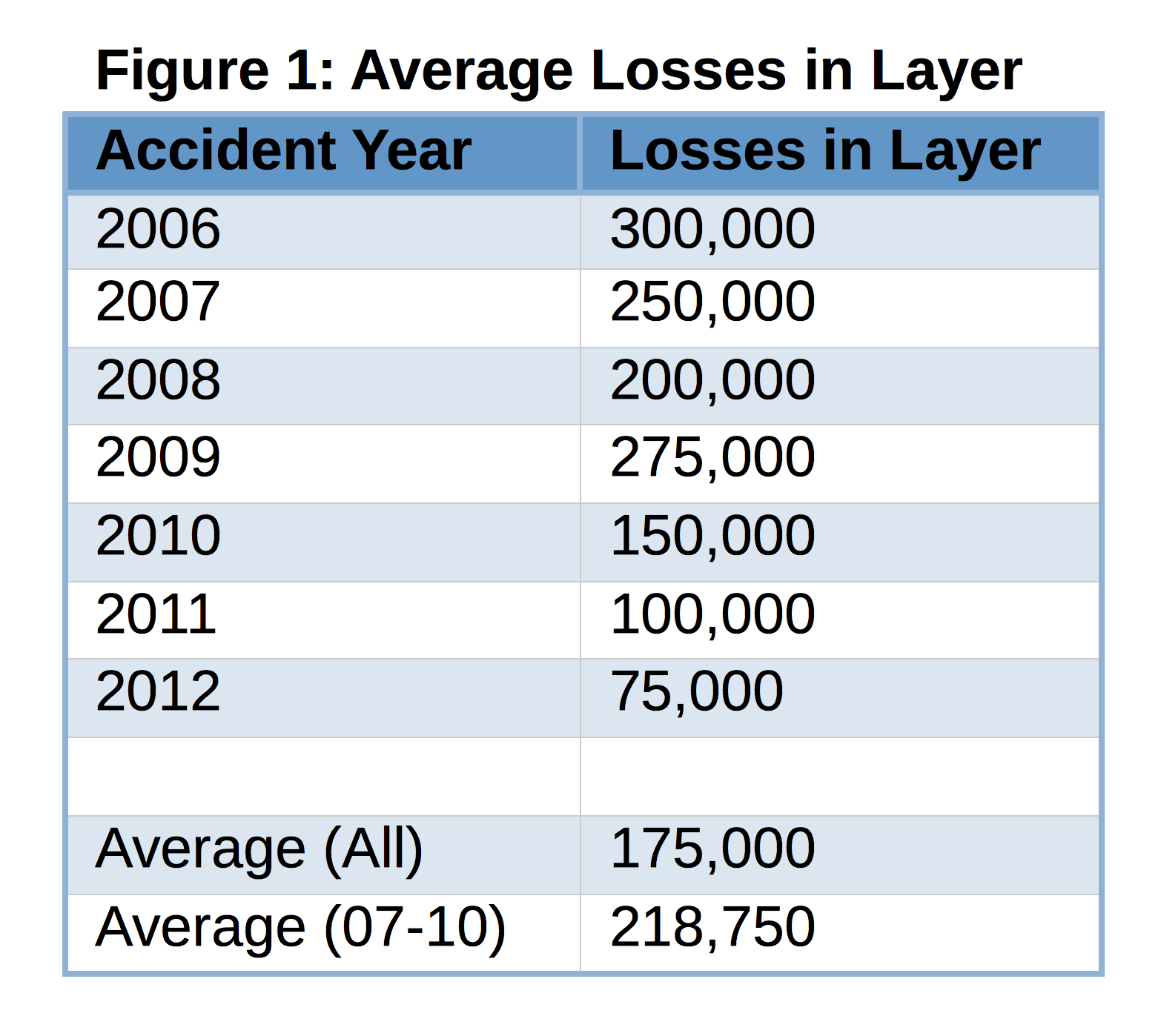
An improvement on this simplistic method is to exclude the two most recent years, as larger claims in those years haven’t had the chance to develop into the higher layers. By removing 2011 and 2012 from the average, the estimate increases to almost $220,000, which is closer to the answers utilizing the additional methods outlined next.

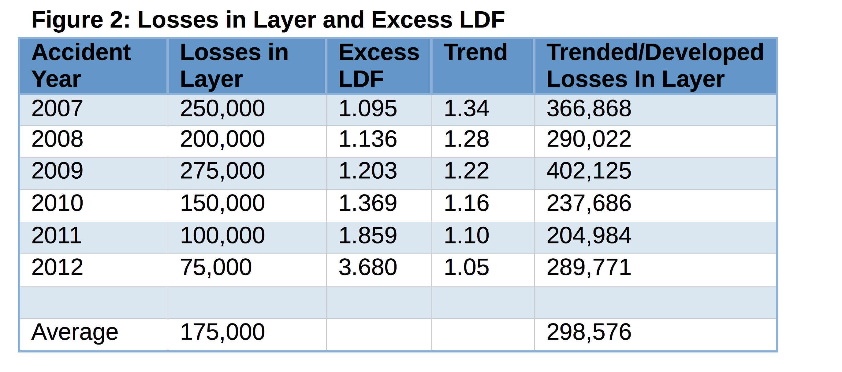
Method 2, while not as simple, does take into consideration loss development and loss trends. The losses incurred in the proposed layer are multiplied by the excess loss development factors (LDFs) and a 5.0 percent loss trend to calculate the ultimate excess losses for the layer $100,000 to $250,000. The results of Method 2 are shown in the table in Figure 2. The average cost of the developed and trended losses is now valued at almost $300,000. Because it is necessary to obtain excess factors and determine appropriate loss trends to apply to the losses in the proposed layer, this method may not be possible, but it does demonstrate the impact that loss development and trends have on the losses. This is the primary reason why Method 1 listed above tends to understate the premium reduction.

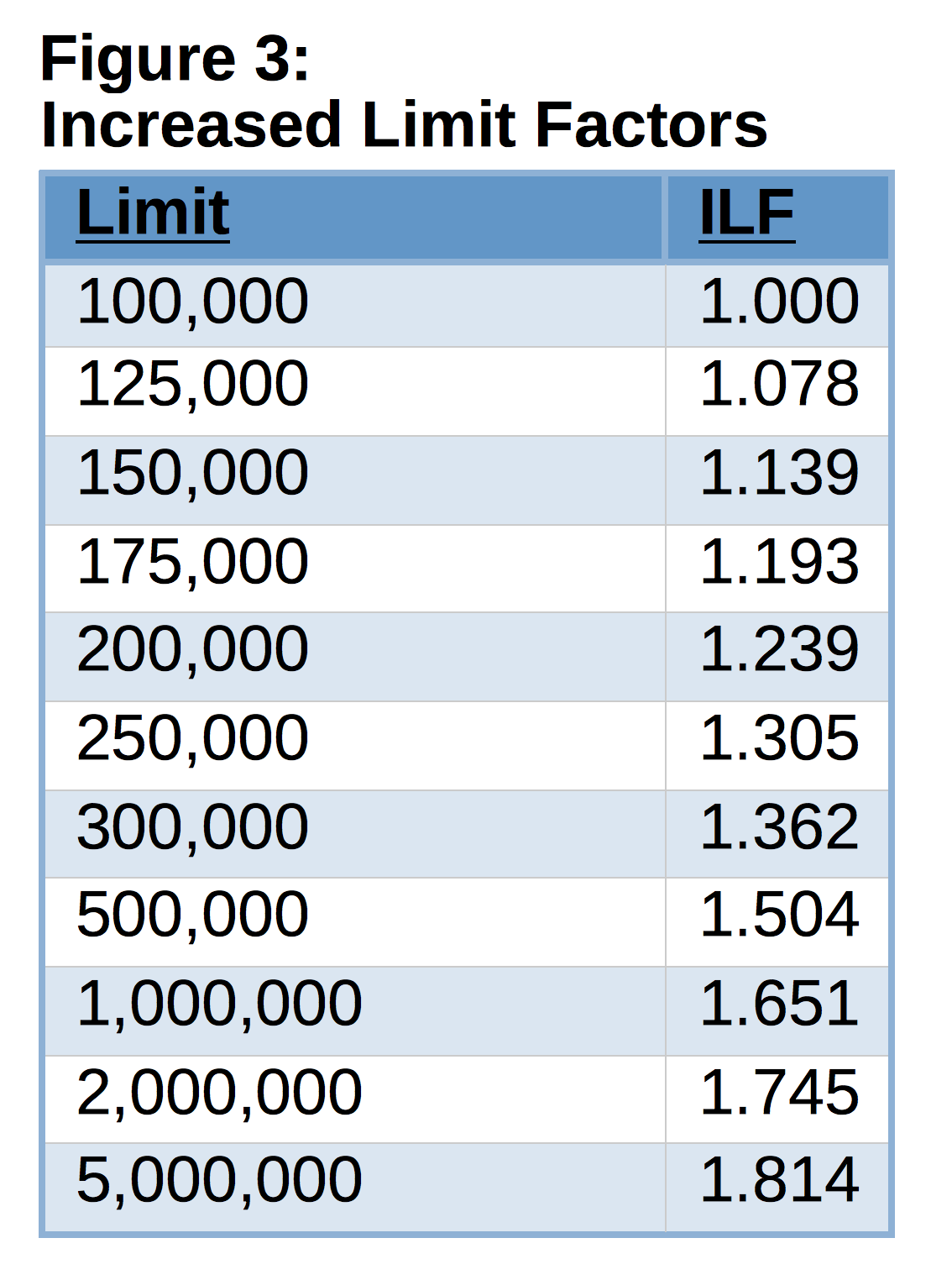
Method 3 utilizes increased limit factors (ILFs) and is more of a theoretical approach than using actual loss data. Typically insurers will limit data to a credible point. For example, a larger program that consistently has several losses that reach $500,000 would likely use its own loss history to price the insurance up to the $500,000 limit and then use industry ILFs to price the remaining coverage at the higher limits on a theoretical basis. A smaller program’s data may only be credible up to the $100,000 limit and then be priced using industry ILFs. The capping of the losses at a credible limit stabilizes the insured’s premium increases and avoids large swings caused by a large fortuitous loss.

Given that ultimate losses have already been calculated for the currently insured policy year at the current retention, the industry ILFs can be utilized to determine the amount of premium charged for the proposed layer. For example, according to Figure 3, if the ultimate loss projection for a program’s current retention of $100,000 per occurrence is $1 million then the estimated ultimate for that program at $250,000 would be $1.305 million ($1 million x 1.305). This method would indicate that the layer between $100,000 and $250,000 is worth approximately $305,000.

Last, Method 4 is the most complicated and would most likely require the assistance of an outside expert. This method relies on a very similar approach to what would be employed in calculating the program’s projected ultimate losses that were used in Method 3. Actuarial methods and the program’s loss data limited to $100,000 are used to determine the program’s ultimate losses at the current retention. Similarly, to calculate the ultimate losses at a $250,000 retention, losses would be limited to $250,000 and plugged into the forecasting models to determine the new projection. In a perfect world, this method would be identical to the answer from Method 3, but because the industry ILFs are not program-specific, this method places more reliance on the program’s actual data for determining the additional layer. However, this method also requires that the program have sufficient data in the proposed layer, otherwise the more theoretical approach is the more prudent approach and a combination of the two should be utilized after determining the appropriate credibility to apply to each method.

Limitations

These methods are a great way to get a ballpark estimate of the premium reduction associated with taking on additional layers of risk, but they are not without limitations.

As mentioned, Method 1 ignores loss development and loss trends.

Method 2 utilizes excess loss development factors which, depending on the layers being priced, are often based on a limited amount of data. This is especially true for the higher layers where the data used to determine these loss development factors is scarce, and the excess factors are based on aggregated industry data that may or may not be a good representation of your unique program. Method 3 also suffers from a similar fate to Method 2, because the increased limit factors are also calculated using aggregated industry data and are not specific to any one program.

Method 4, while being the best method, is hard for most programs to perform without the assistance of an expert.

In addition to the specific limitations of each method, all of them ignore the insurer’s expenses, profits, risk margins, and investment income, which are loaded into the premiums being charged. These methods provide only a pure premium estimate that excludes these loads. Finally, the results of these methods, as with any actuarial estimates, assume that the past is indicative of the future. To the extent that a program has changed significantly, these estimates will not be as reliable.

Conclusion

With this hard market, as with any hard market, the insured will be at the mercy of the insurance market. As business gets tougher to place and prices increase, companies may not have a lot of opportunities to shop around for better prices and may be forced to accept higher retentions and more risk, especially smaller and less sophisticated programs. However, while these methods do have their limitations, they will provide a program’s manager and insurance professional the means of testing the premium reduction for accepting the additional layers and will provide them, at best, the necessary groundwork to negotiate better terms and, at worst, the opportunity to become more sophisticated buyers.

Topics Trends Profit Loss Excess Surplus Pricing Trends Market